radiation superimposed.
NOTE: This document contains many symbols, such as Greek letters, that may not display properly in older browsers. For example, they will not display in Netscape 4.8, but they will in InternetExplorer 6.0. If you see an ampersand followed by the text "alpha" and a semicolon here:
α
instead of the Greek lowercase letter alpha, then your browser is not translating these characters properly.
The purpose of this document is to summarize work conducted since 1998 that has led to the development of several instruments for measuring the transmission of sunlight through Earth's atmosphere. In keeping with the vision originally articulated by the GLOBE Program, the goal of this work has been to help facilitate partnerships among scientists, educators, students, and other non-specialists that will lead both to valuable science and high-quality teaching and learning experiences. (Sadly, this original vision, in which "valuable science" was considered to be at the very heart of teaching and learning science, has been abandoned.)
The document starts with a brief introduction to solar radiation. This is an essential topic for Earth science because any attempt to understand Earth and its atmosphere as a dynamic, interconnected system must begin with an understanding of the sun -- the fundamental source of the energy that drives the system.
Next, there is an introduction to the atmosphere and some of its constituents. Interactions between solar radiation and the atmosphere are important because they provide a way to study atmospheric processes that influence air quality, health, weather, and climate.
Next, there is a discussion of full-sky and direct sun measurements, and broadband and spectral measurements. A large portion of the document describes how to design practical instruments that are both reliable and relatively inexpensive.
Finally, there are two supplementary sections. The first gives equations for calculating solar position, relative air mass, and local solar noon. The second gives a brief introduction to Plancks law for blackbody radiation. These sections are not essential for understanding the rest of the document. However, some knowledge of the sun's position is necessary for the data processing required to convert instrument outputs to physical quantities. Implementing these equations can be tedious, but understanding them requires knowledge of no more than algebra and trigonometry. The equations can be implemented in a computer program or as formulas in a spreadsheet. The introduction to Plancks law may be of interest for secondary school physics courses; it is, after all, one of the most famous equations in all of modern physics.
Although it is important to present science in an age-appropriate way, that is not a primary concern of this document. The level of the presentation may be more appropriate for science educators and other non-specialist adults than for students. It assumes a science background, but not a specialized knowledge of the topics discussed. Hopefully, this document will encourage educators, especially, to develop their own science interests, to build their own instruments for monitoring the atmosphere, and to transmit their enthusiasm to their students.
Stars generate huge amounts of energy through the process of nuclear fusion. Our own sun, an unremarkable medium-sized star, produces a total power E of about 3.9x1026W. This power is radiated into space uniformly in all directions. Fundamental physical laws tell us that the intensity of this radiation decreases as the inverse square of the distance from the sun. The solar constant (So) is defined as the average power per unit area of solar radiation falling on the surface of an imaginary sphere of radius R around the sun:
So = E/(4π R2) = 1370 W/m2
where R is the average Earth/sun distance, about 150,000,000,000 m. The solar "constant" actually fluctuates a little and, the energy the Earth receives varies with the seasonal change in the Earth/sun distance. If one astronomical unit (AU) is the average Earth/sun distance, then the amount of solar radiation reaching Earth varies according to:
Smax = So/(1 - e)2 = So/(0.983)2 = 1417 W/m2
Smin = So/(1 + e)2 = So/(1.017)2 = 1324 W/m2
where e is the eccentricity (a measure of departure from a circle) of Earth's orbit around the sun. Earths eccentricity varies slowly (with periods of hundreds of thousands of years). The current value is about 0.017. The maximum and minimum vary a little more than 3% from the mean. Earth is closest to the sun in early January (yes, really), so this is when maximum solar radiation reaches Earth. The minimum amount radiation is received about six months later.
|
| Figure 1. The extraterrestrial solar spectrum with Planck's law radiation superimposed. |
The radiation leaving the sun on its journey through the solar system is not a completely smooth function of wavelength. Figure 1 shows the extraterrestrial solar radiation, or what an observer would see from a vantage point just above Earth's atmosphere. The irregularities result from processes in the sun's interior and on its surface. For reference, the distribution of equivalent blackbody radiation at 5800 K is also shown. See Section 6 for an explanation of how the blackbody radiation curve is generated
Earth's size and density, and its average distance from the sun, have produced a fortuitous set of circumstances for supporting life as we understand it. Earth's gravity keeps in place an oxygen-rich atmosphere. The average Earth surface temperature (about 16°C), as controlled by the solar constant and the greenhouse effect of the atmosphere, allows water to exist naturally in all its three phases -- solid, liquid, and gas. Although it is almost certainly a mistake to assume that Earth provides a unique environment for the development of life (especially considering that scientists have found primitive life in Earth environments that seem too hostile to support life), it is certainly true that conditions supportive of a permanent oxygen-rich atmosphere and abundant water for most of Earth's long history have made possible the development of advanced forms of life as we understand them.
The atmosphere is made up almost entirely of gases, predominantly nitrogen and oxygen. Table 1 gives the composition of pure dry air near Earth's surface. (See, for example, http://www.arm.gov/docs/education/background/compositionatmos.htm .)
| Gas | Percent by volume (dry air) |
Cumulative percent by volume |
|---|---|---|
| N2 | 78.08 | 78.08 |
| O2 | 20.95 | 99.03 |
| Ar | 0.934 | 99.964 |
| Other trace gases | .036 | 100.000 |
Actual atmospheres contain other naturally occurring and anthropogenic (human-produced) components, as shown in Table 2 [American Chemical Society, 2000].
| Component | Approximate percent by volume (parts per million, ppm) |
|---|---|
| Water (H2O) | 0 4% |
| Carbon dioxide (CO2) | 0.037% (370 ppm) |
| Methane (CH4) | 0.00017% (1.7 ppm) |
| Nitrous oxide (N2O) | 0.00003% (0.3 ppm) |
| Ozone (O3) | 0.000004% (0.04 ppm) |
| Aerosols (liquid and solid particles) | 0.000001-0.000015% (0.01-0.15 ppm) |
| Chlorofluorocarbons (CFCs) | 0.00000002% (0.0002 ppm) |
Although the total amount of these trace components seems very small, except perhaps for water vapor, their effects on the Earth/atmosphere system are profound. The main contribution is the greenhouse effect -- the process whereby some trace gases and aerosols in the atmosphere absorb and re-radiate solar radiation, thereby warming Earth's surface and at least the lower part of its atmosphere. It is not difficult to quantify the overall greenhouse effect. Consider the solar radiation striking Earth. The area of Earth's disk as viewed from space is
area = (πr2) km2
where r is Earth's radius, about 6,378,000 m. Energy from the sun, equal in intensity to the solar constant, is intercepted by Earth's disk, so the total energy incident on Earth is
incident energy = (πr2)So
Not all the incident energy is absorbed because the Earth/atmosphere system reflects part of the energy back to space. The albedo A of the Earth/atmosphere system is the fraction of incoming solar radiation that is reflected by the Earth/atmosphere system, about 0.3. So, the energy absorbed by the Earth/atmosphere system, as viewed from space, is
absorbed energy = (πr2)So(1 - A)
Basic physical laws require that bodies must be in radiative equilibrium. That is, whatever energy is absorbed must be re-emitted in some form. The solar energy striking Earth's disk as viewed from space is re-emitted as thermal radiation by the surface of the entire globe, in an amount proportional to the fourth power of the temperature, as described by the Stefan-Boltzmann Law:
emitted energy = (4πr2)σT4
where 4πr2 is the surface area of Earth and σ = 5.67x10⁻⁸ W/(m2K4) is the Stefan-Boltzmann constant. Set the absorbed energy equal to the emitted energy:
(πr2)So(1 - A) = (4πr2)σT4
Solving for T yields:
T = [So(1 - A)/(4σ)](1/4) = [1370(1-0.3)/(45.67x10-8)](1/4) = 255 K
0ºC = 273 K. So, the temperature at which the Earth/atmosphere system is in radiative equilibrium is about -18ºC. This is very cold from a human perspective -- far below the freezing point of water. But, the average Earth surface temperature is about 16ºC, certainly a more pleasant value from a human perspective. The greenhouse effect accounts for the difference of about 34ºC. Although the temperature of the Earth/atmosphere as viewed from space must still be -18ºC, greenhouse gases warm the lower atmosphere by absorbing some emitted radiation and re-radiating it back to Earth's surface.
A very simple way of accounting for the greenhouse effect is to modify the radiative balance equation:
4σT4(1 x) = So(1 - α)
where "x" is a "greenhouse factor" that provides a measure of how much radiation is absorbed by the atmosphere and re-radiated down to Earth's surface, rather than out to space. For x=0, there is no greenhouse effect. For Earth, a value of x=0.4 produces an equilibrium temperature for the Earth/atmosphere system of about 16°C.
As noted above, the greenhouse effect is essential to support life on Earth. Although there have been large swings in Earth's climate (and its average temperature) during its long history, the rate of global changes have been slow enough to allow many life forms to adapt. Even small changes in the concentrations of trace gases responsible for the greenhouse effect can change both the overall climate and the rate of its change. If the rate of change is too rapid, then species may not be able to adapt; this is the primary source of concern about human-induced changes in greenhouse gases. Table 3 shows the relative efficiency of some greenhouse gases [American Chemical Society, 2000]. CO2 is arbitrarily given an efficiency of 1.
| Greenhouse gas | Relative effectiveness |
|---|---|
| Carbon dioxide (CO2) | 1 (arbitrarily assigned) |
| Methane (CH4) | 30 |
| Nitrous oxide (N20) | 160 |
| Water (H2O) | 0.1 |
| Ozone (O3) | 2000 |
| Trichlorofluoromethane (CCl3F) | 21,000 |
| Dichlorodifluoromethane (CCl2F2) | 25,000 |
Water vapor is the most prominent greenhouse gas, and its relatively low greenhouse effect efficiency is overridden by its much higher concentration in the atmosphere. Carbon dioxide is also a potent greenhouse gas even at the concentration shown in Table 2. CO2 has both natural and anthropogenic sources, and is of great concern because steadily increasing CO2 levels due to the burning of fossil fuels since the start of the Industrial Revolution are generally believed to be warming Earth's climate more quickly than at any time in the known past.
The most notorious trace gases belong to the family of chemicals known as chlorofluorocarbons (CFCs). These have no natural sources and have entered the atmosphere only as the result of human industrial activity -- because of their chemical stability, they have been used as coolants and propellants in spray bottles. In addition to being potent greenhouse gases, and even at what appears to be miniscule concentrations, CFCs are primarily responsible for dramatic seasonal reductions in concentrations of stratospheric ozone in the upper atmosphere (the now-famous "ozone holes"). T his is a problem because stratospheric ozone is "good ozone" that protects Earth's surface from ultraviolet (UV) radiation that can have harmful effects on humans and other organisms. (The "bad ozone" near Earth's surface, which is a pollutant that can cause serious health and environmental problems, is not affected in this way because it is produced locally as a result of photochemical processes at Earth's surface.)
Even seemingly small changes in the concentrations of the more potent greenhouse gases, especially if they occur quickly, have the potential to disrupt entire ecosystems that thrive only within a narrow range of environmental conditions.
Monitoring Earth's atmosphere is a challenging task. In industrialized countries, there are well-established networks of instruments to monitor the atmosphere close to Earth's surface. Some stations are used for scientific purposes, but most serve a primarily regulatory function -- monitoring a specific set of air quality indicators as mandated by government agencies. (In the U.S., the "criteria pollutants" on which the Air Quality Index is based, as established by the Environmental Protection Agency, are SO2, NO2, O3, CO, and particulates. Although these quantities are certainly of scientific interest, they are only local measurements and represent only a small subset of important atmospheric components.
In order to understand how the Earth/atmosphere system works, it's necessary to understand the entire atmosphere, not just the part within direct reach from Earth's surface. Typically, the total amount of gases and particles in a column of atmosphere cannot be determined from measurements just at Earth's surface -- by a single measurement essentially at the bottom of the atmosphere column. Balloons, airplanes, and rockets are all used to perform direct measurements in the atmosphere at altitudes up to and beyond the stratosphere. Satellite-based instruments provide global views, but it is difficult to infer surface and column distributions from space-based measurements; such measurements must still be supplemented by ground-based measurements.
An important way of probing the atmosphere from the ground is to measure the effects of the atmosphere on sunlight transmitted through the atmosphere to Earth's surface. These indirect techniques provide information about the entire atmosphere above the observer, not just the atmosphere that can be sampled directly. Such upward-looking measurements are especially valuable when they are compared with downward-looking measurements from space. Many of these ground-based measurements are not difficult, and are well within the capabilities of students and other non-specialists.
Not all solar radiation reaching the top of the atmosphere reaches Earth's surface. As noted previously, an average of about 30% is reflected back to space by the atmosphere, surface, and clouds. Within the atmosphere, some radiation is scattered or absorbed. Part of the scattered radiation returns to space. Absorbed radiation is eventually re-emitted, but at different wavelengths. Some of this re-emitted radiation also returns to space. The total amount of solar radiation reaching Earth's surface is called the insolation, or solar irradiance.
Figure 2 shows the spectral distribution of insolation for a so-called standard atmosphere -- an "average" atmosphere with specified characteristics -- compared to the extraterrestrial radiation at the average Earth/sun distance. Insolation consists of two basic parts: radiation directly from the sun and diffuse radiation from the rest of the sky. The relationship between direct and diffuse radiation depends on the position of the sun in the sky. The sun in Figure 2 is at an elevation angle of about 42º, giving a relative air mass of about 1.5. (If the sun is directly overhead, the relative air mass is 1, by definition.)
 |
| Figure 2. Direct, diffuse, and total insolation for a standard atmosphere, with relative air mass of 1.5. |
The fact that diffuse radiation is a significant part of total insolation offers an important clue about what happens in the atmosphere: molecules scatter sunlight. Some of the scattered light is directed back to space and some of it reaches Earth's surface. As a result, the sky itself appears to be a source of light even though all the radiation originally comes just from the sun. (Beyond the atmosphere, there is no diffuse sunlight. This is why "space" appears black.)
Scattering of light by molecules is called Rayleigh scattering after the British physicist John William Strutt, the third Baron Rayleigh (1842 1919) who first described this phenomenon mathematically. The fact that molecules scatter blue light more efficiently than light with longer wavelengths explains why the sky appears blue. The fact that red light is scattered less than blue and other colors of light explains why the sun appears more and more red as it approaches the horizon. As particles get larger, scattering becomes less wavelength-dependent. Clouds appear white because the large water droplets in clouds scatter and reflect light uniformly throughout the visible range of wavelengths.
Solar radiation is not just scattered as it passes through the atmosphere. Some radiation is absorbed by molecules and particles and re-emitted as thermal radiation. The nature of molecular bonds permit the absorption of radiation at specific wavelengths. As a result, insolation is not just a diminished version of the extraterrestrial radiation. Instead, there are "holes" in the insolation spectrum caused by molecular absorption.
Water vapor is the major absorber -- hence its importance as a greenhouse gas. Its most prominent absorption occurs far out in the infrared part of the solar spectrum, but there are also absorption bands in the near-IR around 720, 820, and 940 nm. The effects of water vapor absorption are clearly visible in Figure 2.
The second most important absorber in the UV-visible-Near-IR part of the spectrum is ozone. It has a deep bell-shaped absorption band between 210-310 nm (the Hartley band), and less prominent structured bands between 310-350 nm (Huggins band) and 450-850 nm (Chappuis bands). Ozone absorbs almost all UV-C radiation (200-280 nm) and roughly 70% or more UV-B (280-320 nm) radiation. There is little atmospheric absorption of UV-A radiation (320-400 nm). (The ozone bands are not clearly visible at the resolution of Figure 2.)
In addition to molecular scattering, larger particles in the atmosphere, called aerosols, also scatter sunlight. This is called Mie scattering, after the German physicist Gustav Mie (1868 - 1957) who first described this phenomenon mathematically. These particles have sizes in the same range as the wavelength of light (~100-1000 nm), so they scatter light differently than molecules, which are much smaller.
The effects of scattering and absorption enable scientists to develop ground-based measurement strategies based on this important observation:
There are two general categories of instruments used to measure the transmission of sunlight through Earth's atmosphere: instruments that measure radiation from the entire sky, and instruments that measure only direct solar radiation. Within each of these categories, instruments can be further subdivided into those that measure radiation over a broad range of wavelengths and those that measure only specific wavelengths.
As their name implies, full-sky instruments need an unobstructed view of the entire sky. So, they need sites that have a 360º view of the horizon, without significant obstacles. Corrections can be made for limited horizon obstructions but, the more clear the horizon is, the more accurate measurements will be.
A less obvious requirement for full-sky detectors is that they have good "cosine response" to direct sunlight. If sunlight has intensity Io when the sun is directly above a horizontal surface (zenith angle of 0º), then the intensity Iz at some other zenith angle z is
Iz = Iocos(z)
If an ideal detector on a horizontal surface is illuminated by direct light, then its response should be proportional to the cosine of the zenith angle of the light source. Real detectors do not have perfect cosine response. Cosine response corrections can be determined and applied for a direct light source, but this issue becomes much more complicated especially under partly cloudy skies, when the radiation incident on a detector is an unknown combination of direct sunlight and diffuse sky radiation, as is the case for full-sky solar radiation.
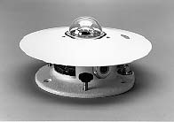 |
| Figure 3. Eppley PSP pyranometer. |
As their name implies, these instruments are designed to view only light coming directly from the sun. The radiation incident on one or more detectors is restricted to a narrow cone of the sky, the instrument's field of view. The field of view should be as small as possible in order to restrict the amount of scattered light that finds its way to the detector, while still providing enough light for the detector to produce a usable output signal.
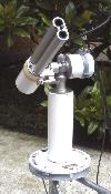 |
| Figure 4. CIMEL sun photometer. |
Broadband detectors are required for measuring total solar radiation. This is not as easy as it might seem, basically because solar radiation covers such a broad range of the electromagnetic spectrum. (Recall Figures 1 and 2.)
High-quality reference pyranometers, such as the Eppley pyranometer shown in Figure 3, use thermopiles -- collections of thermocouples. Thermocouples consist of dissimilar metals mechanically joined together. They produce a small current proportional to their temperature. When thermopiles are appropriately arranged and coated with a dull black finish, they serve as nearly perfect "black body" detectors that absorb energy across the entire range of the solar spectrum. These instruments are very expensive (several thousand dollars) and not suitable for routine field work, whether by students or professionals.
An inexpensive alternative is to use photovoltaic detectors. Silicon-based solar cells are an obvious choice. Their major disadvantage is that their spectral response is different from the solar spectrum. Typically, they respond to sunlight in the range from 400 to 1100 nm, with a peak response in the near-infrared, around 900 nm. This restricted spectral response represents a subset of the solar spectrum which, under normal outdoor sunlight conditions, introduces a potential error of a few percent. However, reliable and inexpensive solar radiation monitors are so desirable that a great deal of research effort has been dedicated to designing and understanding silicon-based pyranometers. (See, for example, King and Myers [1997].) Commercial pyranometers that use silicon-based detectors -- they might more accurately referred to as "surrogate" pyranometers -- are much less expensive than thermopile-based pyranometers (a few hundred dollars), and it is possible for educators and students to build a solar cell-based pyranometer for much less (a few tens of dollars) than of the cost of commercial instruments. Such an instrument might be less rugged, or have a different cosine response than a commercial instrument, but it is identical in principle.
For both sun photometers and full-sky instruments, some measurements require detectors that respond only to a specific range of wavelengths. For research instruments the first choice for spectrally selective detectors are relatively broadband photodetectors used in combination with so-called interference filters that transmit only a limited range of wavelengths -- often only a few nanometers or less. These detectors are expensive, fragile, and subject to unpredictable degradation. Thus, even in the visible part of the spectrum, they are not a good choice for student instruments. Detectors for the shorter UV wavelengths and for IR wavelengths beyond 2000 nm or so tend to be very expensive, with no inexpensive alternatives. These realities impose some important practical limitations on the kinds of spectrally selective measurements that can be made with inexpensive instruments. Nonetheless, there is a great deal of useful and interesting atmospheric science that can be done with the instruments described below, which lie within the range of roughly 350-1000 nm -- most of the UV through the visible and near-IR parts of the solar spectrum.
The first atmosphere monitoring instrument developed for the GLOBE Program used light emitting diodes (LEDs) as detectors. The physical laws that cause LEDs to emit light when a current is passed through them also cause LEDs to generate a small electrical current when light in an appropriate wavelength range shines on them. LEDs are inexpensive, stable, and virtually indestructible -- essential attributes for instruments intended for student use.
Of course, LEDs have some disadvantages. The main difficulty is that even though LEDs can serve as spectrally selective light detectors, they are designed to emit light, not detect light, and they are optimized for their intended purpose. The spectral response of LEDs is often wider than is desirable for certain kinds of atmospheric measurements, and the wavelength ranges may not be ideal for the intended measurement. Also, the spectral response of LEDs is not simply related to its emission spectrum. The current generated by an LED when it is exposed to light is sensitive to changes in temperature and this can limit its usefulness if there is a strong temperature dependence. However, despite the fact that this application is far removed from the intended use of LEDs, there are still several scientifically valid applications of LED detectors in the UV, visible, and near-IR.
Within the range of detector possibilities discussed above, there are several scientifically valuable measurements that can be made.
 |
| Figure 5. 4-day mean insolation over North America, late December, 2003, based on GOES visible images. |
As noted above, insolation at Earth's surface (the total solar irradiance, in units of W/m2) is a fundamental measurement for understanding Earth and its atmosphere as an interconnected dynamic system. There are also obvious engineering applications of such a measurement, for designing and siting solar power arrays. From a science perspective, long-term solar monitoring helps scientists understand persistent changes in the atmosphere.
Figure 5 shows modeled 4-day mean insolation over North America in late December, 2003, based on analysis of GOES visible images [Diak, Bland, and Mecikalski, 1996]. The units are megajoules per day.
There are also less obvious applications for an insolation monitor. For example, within a theoretical envelope provided by the diurnal solar cycle under clear skies at a specified time of year, site latitude, and elevation, it may be possible to relate temporal and spatial fluctuations of insolation to air quality and cloud cover. Weather-related variability in insolation is evident in Figure 5. A local view of weather-related variability is shown in Figure 6, which is taken from a larger set of pyranometer data recorded since September 2004 at 1-minute intervals at Central Middle School, Waterloo Iowa. In these data, the effects of clouds moving across the observing site are clearly evident, including the phenomenon by which sunlight reflected from the sides of clouds can temporarily increase the amount of insolation reaching the surface over what would be seen under a clear sky
 |
| Figure 6. Insolation during June, 2004, at Central Middle School, Waterloo Iowa |
As noted above, molecules and liquid or solid particles suspended in the atmosphere (aerosols) scatter and absorb sunlight. The effect of molecular scattering on direct sunlight can be calculated theoretically, as a function of wavelength, as can absorption by gases. The remaining reduction at a particular wavelength is due to scattering and absorption by aerosols in the atmosphere. Reductions in transmission are described by a quantity known as optical thickness, or optical depth. The more scattering and absorption reduce transmitted sunlight as viewed along a direct path, the larger the optical thickness. The basic equation governing the transmission of radiation through an intervening medium (the Lambert/Beer/Bouaguer Law) is
Iλ = Io,λexp(-αλm)
where Io,λ is the original source intensity, Iλ is the intensity after radiation passes through a medium of thickness m, and αλ is the total atmospheric optical thickness, all at wavelength λ. A perhaps more intuitive formulation describes the same effect in terms of percent transmission through the atmosphere T:
T = 100·exp(-αλ)
The relationship between percent transmission and optical thickness is shown in Figure 7. A typical value of total optical thickness for visible light in clean air is around 0.2, or 81.9% transmission.
| Figure 7. Percent transmission through the atmosphere vs. total optical thickness. |
The total atmospheric optical depth αλ consists of three basic parts: molecular (Rayleigh) scattering by the atmosphere, atmospheric absorption by gases such as ozone, and scattering by aerosols (aerosol optical thickness, or AOT):
αλ = αλ,R + αλ,g + αλ,a
The strongly wavelength-dependent contribution of Rayleigh scattering can be calculated using theoretical models of the atmosphere. For practical calculations, a parameterized model is used. One formulation has been given by Bucholtz [1995]:
αλ,R = (p/po)A·λ·(-B - C·λ - D/λ)
where (p/po) is the ratio of actual barometric pressure at an observing site to standard pressure at sea level (1013.25 mbar), &lambda. is the wavelength in units of micrometers. The coefficients A, B, C, and D given in Table 4 are empirically derived values that provide a mathematical best fit to theoretical calculations:
| Coefficient | λ≤0.500 μ (500 nm) | λ>0.500 μ (500 nm) |
|---|---|---|
| A | 6.50362 x 10⁻³ | 8.64627 x 10⁻³ |
| B | 3.55212 | 3.99668 |
| C | 1.35579 | 1.10298 x 10⁻² |
| D | 0.11563 | 2.71393 x 10⁻² |
Figure 8 shows the Rayleigh coefficient at sea level as a function of wavelength.
 |
| Figure 8. Dependence of the Rayleigh scattering coefficient upon wavelength. |
The predominant gas absorber over the wavelength range of interest for these instruments is ozone. Figure 9 shows the climatological mean optical thickness for ozone across visible and near-IR wavelengths [Leckner, 1978; Bird and Riordan, 1984]. It is small (<0.04), but can be significant for clean air with small values of aerosol optical thickness.
 |
| Figure 9. Ozone optical thickness at visible and near-IR wavelengths. |
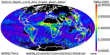
Sources of aerosols include volcanic activity, dust from deserts and agricultural activity, sea spray, and air pollution. The amount of aerosols varies widely around the globe, and there are strong seasonal effects. In clean skies, AOT at visible wavelengths will be less than 0.1. Figure 10 shows an 8-day mean of global aerosol optical thickness from early November, 2003, as calculated from data recorded by the Moderate Resolution Imaging Spectroradiometer (MODIS) instrument on NASA's EOS/Terra and Aqua spacecraft. Cloudy weather and/or snow cover over the northern hemisphere prevent AOT calculations from being done. Bright land surfaces, such as the Sahara Desert and the Saudi Arabian Peninsula, and permanently snow/ice-covered polar regions, are inaccessible to MODIS aerosol retrievals. Thus, ground-based measurements are still very important.
High values of AOT resulting from biomass burning activity are clearly evident in sub-Saharan Africa and the Amazon Basin in South America. Even though aerosols directly over the Sahara are not visible to MODIS, a plume of Saharan dust is visible over the Atlantic Ocean, blowing westward. It is common for Saharan dust to find its way to the Western hemisphere. More recently, it has also become clear that large amounts of dust and other pollution are often blown eastward from Asia to the west coast of the United States.
 |
| Figure 10. 8-day mean aerosol optical thickness from MODIS/Terra, early November, 2003. |
Photosynthetically active radiation (PAR) refers, as its name implies, to that subset of total solar radiation that plants use for photosynthesis. Typically, this is a full-sky measurement. The spectral definition of PAR is not precise, because different kinds of plants respond to different parts of the solar spectrum. However, PAR is generally considered to include just the visible part of the solar spectrum -- between 400 and 700 nm. Thus, a PAR detector is similar to a pyranometer, but with its spectral response limited to just visible wavelengths.
Although it is typically true that the output from a full-sky PAR detector is somewhat correlated with total solar radiation, the correlation is imperfect enough that scientists require a separate measurement for PAR radiation. This is extremely important in agriculture and botany, for studying plant behavior under different lighting conditions -- under crop or tree canopies, for example.
Whereas insolation is reported in units of energy density (W/m2), PAR radiation is reported in terms of the total number of photons in the energy between 400 and 700 nm. This makes sense because photosynthesis involves the interaction between individual photons and molecules. Specifically, PAR is reported as the number of moles of photons per unit area, per second, in the spectral interval from 400 to 700 nm, where there are 6.0222 x 10²³ (Avogadro's number) photons per mole.
Figure 11 shows PAR from the USDA UV-B Monitoring Network at Beltsville, Maryland, on 1 September, 2006.
 |
| Figure 11. Photosynthetically active radiation (PAR) at Beltsille, Maryland, 1 September, 2006. |
Total atmospheric water vapor, also called total column water vapor or total precipitable water vapor (PW) is defined as the thickness of a layer of water obtained by condensing all the water vapor in a column above the observer and bringing it down to the observer's elevation. Typically, PW is a few centimeters.
PW is distributed unevenly around the globe. Figure 12 shows a view of the Western hemisphere on 22 December, 2003, based on infrared (6750 nm) data from the GOES-12 satellite. In general, there is more water vapor over warm water and equatorial forests because of evaporation and transpiration. Not surprisingly, there is much less water vapor over deserts and at high elevations. Although it is commonly believed that there must be a lot of precipitation at the poles, because they are covered with snow and ice, the air over Earth's polar regions is usually very dry.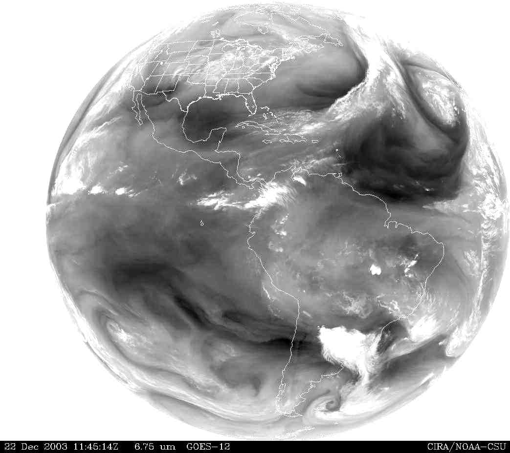 |
| Figure 12. GOES-12 6750 nm water vapor image for the Western hemisphere, 11:45 UT, 22 December, 2003. |
At a given location, PW varies seasonally and diurnally. Long-term global changes in PW can signal climate change. Figure 13 shows a 12-year record of PW over Seguin, Texas, USA [Mims, 2002].
 |
| Figure 13. Precipitable water over Seguin, Texas, USA. |
As noted above, radiation from the sun covers a wide range of the electromagnetic spectrum. Ultraviolet radiation, with wavelengths just below the visible spectrum, is especially important to life on Earth. The UV spectrum is usually defined as radiation with wavelengths between 100 and 400 nm. There are three widely used UV categories, as shown in Table 5.
| UV Category | Wavelength Range(nm) |
|---|---|
| UV-A | 315-400 |
| UV-B | 280-315 |
| UV-C | 100-280 |
UV-C radiation can damage DNA. It will kill bacteria and viruses. In fact, artificial UV-C sources are used to sterilize medical equipment and to purify air and water. There is essentially no naturally occurring UV-C radiation at Earth's surface because it is absorbed by oxygen in the atmosphere. The interaction of UV-C radiation with oxygen is the source of stratospheric ozone.
UV-B is partially absorbed by ozone in the atmosphere. It is considered a destructive form of UV radiation at Earth's surface because it can damage living tissue and manmade materials. Increasing exposure to UV-B radiation from sunlight produces sunburn and is widely accepted as the cause of increasing rates of the most serious forms of skin cancer (melanomas). Even though overexposure to the sun is a serious human health problem, "getting a tan" is still considered important by many light-skinned individuals. Because UV-B is only partially absorbed by ozone, even a small decrease in the amount of stratospheric ozone can significantly increase the risk of skin cancer for light-skinned humans. Overexposure to UV-B is also associated with eye diseases such as cataracts, which can affect humans regardless of their skin color.
Low energy UV-A ("black light") sources can cause some materials to emit visible light (fluoresce), which makes them appear to glow in the dark. UV-A radiation penetrates farther into human skin then UV-B. Tanning lamps are designed to produce UV-A rather than UV-B radiation because exposure to UV-A will darken light skin without burning. However, UV-A exposure can cause premature skin aging and eye problems. Therefore, health professionals warn against excessive UV exposure, including UV-A, no matter what the source.
Because of its intimate connection with the concentration of stratospheric ozone ("good" ozone), UV radiation is of great scientific interest. At ground level, UV has some important ecological effects. To cite just two examples, UV radiation influences the breeding patterns of potentially harmful insects such as mosquitoes, and some animals, including insects, can see UV light that is beyond the response of the human eye.) Although UV radiation is of special concern because overexposure is a serious public health problem, it is important to understand that the interactions of UV radiation with life on Earth are complex and, in many cases, poorly understood. UV radiation is inherently neither "good" nor "bad." Life on Earth has evolved within a particular radiation environment that includes some UV radiation. Disruptions to this radiation environment, causing some forms of radiation to increase or decrease, can have serious and unforeseen consequences -- this is the source of concern about "ozone holes" in the stratosphere.
Each of the instruments discussed in this section shares a common underlying physical principle. When solar radiation strikes a light-sensitive detector (photodetector), atoms in the detector absorb some of the energy (from photons). In this excited state, which may be produced only by light in a specific range of wavelengths, the atoms release electrons, which can flow through a conductor to produce an electrical current. The current is proportional to the intensity of the radiation striking the detector.
Some of the instruments discussed here use light emitting diodes (LEDs) as detectors. These devices are intended to work the other way around, as light emitters. When an electric current flows though an LED (in the form of an electrical current), atoms in the LED "chip" drop from an excited state to a less excited state and release energy in the form of radiation. Typically, this radiation is in the visible part of the spectrum, but some LEDs emit UV or IR radiation.
It is perhaps not obvious that LEDs will also work as spectrally selective photodetectors. However, just like other photodetectors, LEDs respond to light in a specific wavelength range by generating a flow of electrons. The current produced by an LED used as a light detector is extremely small -- too small to be measured directly with inexpensive equipment. The problem can be solved by converting the current to a voltage and amplifying it. This task is easily accomplished with a special amplifier configuration called a transimpedance amplifier. These devices are inexpensive and easy to design using a standard operational amplifier (op amp) with only a few additional components.
 |
| Figure 14. Generic emerald green LED emission compared to measured spectral response. |
The spectral distribution of an LED's emitted radiation is not the same as its response spectrum. The emission spectrum is readily available from the manufacturer, because this is fundamental information required to select an LED for use as a light source. Information about the response spectral distribution is rarely available, because it is typically of no interest to the purchaser of an LED. So, the response spectrum must be measured in order to determine the suitability of an LED as a light detector for a particular application. The peak response wavelength is invariably lower than the peak emission wavelength but, as a practical matter, it is not possible to predict the location and shape of the response spectrum based on the emission spectrum. Figure 14 shows the normalized generic emission spectrum of a typical "emerald green" LED, as supplied by its manufacturer, compared to its normalized directly measured response spectrum. According to these data, the emission peaks at about 555 nm, but the peak response is around 530 nm.
A basic silicon-cell based pyranometer is an extremely simple device. Figure 15 shows a circuit diagram for two cells connected in parallel to a direct-current (DC) milliammeter. Unlike LED detectors used in other instruments described here, solar cells are designed specifically to convert solar radiation to a flow of electrons as efficiently as possible. As a result, even a very small solar cell in bright sunlight will produce a current large enough to be measured with an inexpensive ammeter. More than one cell is shown in Figure 15 because a single cell may not provide enough current to drive a particular analog meter over a useful range. (Cells connected in parallel produce more current. Cells connected in series produce higher voltages.)
 |
| Figure 15. Circuit diagram for a simple solar-cell based pyranometer. |
Figure 16 shows a pyranometer that uses two small solar cells. The white disk on the left-hand side of the off-white enclosure is a thin piece of Teflon® to diffuse sunlight incident on the small solar cells below. A small "bullseye" level is mounted on the right-hand side of the enclosure. (It is important for pyranometers to be mounted as precisely horizontal as possible.) The dark object attached to the black cable is a commercial photovoltaic pyranometer used for calibrating the instrument. Output from the solar cells is connected through the gray cable to an analog milliammeter mounted in the blue enclosure. These solar cells produce about 0.5 mA in full sunlight.
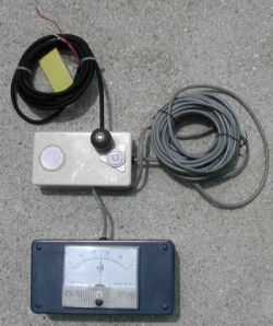 |
| Figure 16. A solar-cell based pyranometer with an analog current meter, shown with a commercial pyranometer used for calibration. |
This simple instrument can be used to demonstrate a great deal not only about solar radiation, but also about the underlying principles of electromagnetism that allow flowing electrons to provide the power required to rotate the meter mechanism.
There are some subtleties involved in designing a solar cell pyranometer (and other photovoltaic devices), and the details are interesting from the perspective of teaching physics. Silicon solar cells are semiconductor devices consisting of thin sheets of silicon "doped" with impurities. In solar cells, two dopants are used -- one has an excess of electrons (a negatively charged, or N-type dopant) and the other has a deficit of electrons (a positively charge, or P-type dopant). This doping creates an electric field. When light strikes the cell, the energy from individual photons is absorbed by atoms. This results in the release of electrons, which flow from the N-type material to the P-type material and create a potential difference.
The potential difference -- the voltage -- measured across the terminals of a solar cell, without connecting a resistive load across the cell, is called the "open circuit" voltage. A solar cell will produce very nearly its maximum open circuit voltage when exposed to even a little sunlight. Figure 17 shows open circuit voltage as a function of solar radiation. These data were collected on a day when cumulus cloud cover ranged from scattered to broken and even overcast in the afternoon. Even under these highly variable conditions, the voltage remains essentially constant until late in the afternoon. The fact that very little insolation is required to produce nearly the maximum open circuit voltage -- voltage is essentially independent of insolation over a wide range of insolation values -- means that open circuit voltage cannot be used as a measure of insolation.
 |
| Figure 17. Solar cell voltage as a function of time (variable cloud cover). |
Under open circuit conditions, electrons do not flow through the solar cell. To put it another way, it is one thing to "separate" electrons to create a potential difference (a voltage), but quite another thing to produce a flow of electrons that can perform useful work (in the physics sense of this term). It is the quantity of flowing electrons that provides the ability to do work and it is the flow of electrons that is proportional to the intensity of the radiation falling on a detector.
Based on Ohm's famous law, voltage = current x resistance (V=IR), it is tempting to place a resistor across the terminals of a solar cell so that electrons will flow. Then a voltage can be measured directly across the resistor without using a transimpedance amplifier as described at the beginning of Section 4. Indeed, some photovoltaic pyranometers do just that.
The potential problem lies with the limited ability of a solar cell to produce electrons. Electrical power equals current times voltage (P = IV). The ability of a solar cell to provide this power is limited by its size. This is why solar cell specifications often say something like, "12V at 100 mA." This means that the solar cell can be expected to provide a power of 1.2W to a device that requires an operating voltage of 12V at a current of about 100 mA. The open circuit voltage will be higher than 12 V. When the load on the cell is increased, by reducing the resistance of the device (that is, by increasing the current demand of the device), then the voltage will drop because the supply of electrons is insufficient to meet the demands of this task.
Figure 18 shows current and voltage output from a small solar cell under conditions of relatively constant insolation. One set of data is for an overcast day and the other is for a cloud-free day. Both data sets were collected during the winter, so the insolation is far below its maximum expected values in the summer. Because the active surface area of this solar cell is only few square millimeters, its current output is limited to a few hundred microamps even in bright sunlight.
 |
| Figure 18. Current and voltage as a function of load resistance for a small solar cell. |
Over a certain range of resistive loads, the current output remains constant and voltage across the a fixed resistor within this range is linearly related to the current; that is, if the solar irradiance doubles, the voltage doubles. The maximum load for which the output will remain linear depends on the maximum amount of insolation -- the higher the maximum insolation, the smaller this load must be. At some point (above a load of about 900 ohms for trial 2), the current starts to drop, as the ability of the cell to produce electrons is limited. This effect can be visualized in terms of traffic flow, with the size of a highway (the number of lanes, perhaps) being equivalent to the inverse of the resistive load. Suppose a very wide highway can easily handle a flow of C cars per hour. If C isn't too large, then a smaller highway can also handle this load. However, at some point a highway could become so small that it can no longer support a flow of C cars per hour. The resulting congestion -- a slowing down of traffic -- is equivalent to a reduced current.
When a solar cell is used as a pyranometer, the same limitations apply. If the power required to maintain a voltage V across a resistance R exceeds the ability of the solar cell to provide the required electrons, then the voltage across the resistor will no longer be proportional to the solar radiation falling on the cell.
There is yet another important design consideration that applies to all full-sky instruments. As mentioned previously in Section 2.1, the response of full-sky detectors to direct radiation should vary as the cosine of the zenith angle of the radiation. Figure 19 shows the response of three different pyranometers: an Eppley Model 8-48 pyranometer, a LI-COR pyranometer, and a homemade solar cell pyranometer. Note the "cosine-like" shape of the data, especially on clear days, and contrast this to the graph of open circuit voltage previously shown in Figure 15.
In Figure 19, the Eppley pyranometer (by far the most expensive) is taken as the reference. The LI-COR data are based on the calibration supplied by the manufacturer. The solar cell instrument is calibrated against the Eppley by minimizing the overall difference between the results over an extended period of time.
 |
| (a). Solar insolation during January 1999. |
 |
| (b). Solar insolation during July 1999. |
| Figure 19. Solar insolation comparisons with three different pyranometers,
Philadelphia, Pennsylvania, USA (lat = 39.96N, lon = 75.19W). |
Figure 19 shows that the homemade solar cell pyranometer performs about the same as, and certainly no worse, than the commercial LI-COR instrument (which is also a photovoltaic-based instrument). Note that, on clear days, the LI-COR values are higher than the Eppley values in the winter and lower in the summer. As currently calibrated, values from the homemade pyranometer are always a little less than those from the Eppley on clear days. The difference is larger during the winter than during the summer. There are several reasons why the calibrations cannot be made to match under all conditions. The differences are at least partly due to differences in cosine response; the Eppley's cosine response is better than either of the other two. The spectral response of the Eppley instrument (a thermopile instrument) is different from the solar cell-based instruments. It is also likely that the response of the solar cell in this homemade pyranometer degraded somewhat between January and July, as it was not protected by a diffuser and it was a type of solar cell (thin film amorphous silicon) that is known to have degradation problems.
The peak response of the homemade instrument relative to the Eppley can, of course, be adjusted by increasing the calibration constant. Note, however, that as currently calibrated, values from the homemade pyranometer on cloudy days in July exceed those from the Eppley, so increasing the calibration constant to match better on clear days would make the agreement worse for cloudy days. This discrepancy is due primarily to differences in spectral response -- a cloudy sky is a different color than a clear sky, so calculated values of insolation will be different with detectors having different spectral responses.
The differences between results from a high-quality pyranometer and photovoltaic "surrogate" pyranometers may already be small enough to yield sufficiently accurate data for some purposes, especially when insolation is averaged over a day. In any event, the discrepancies cannot be removed simply by changing a single calibration constant. It may be possible to develop algorithms to reduce the differences, for example, by taking into account the minimum solar zenith angle on a particular date (which affects the impact of imperfect cosinse response) and by modifying the calibration constant depending on the "noise" in the insolation data for a particular day. Clear skies are less noisy than cloudy skies.
A sun photometer for measuring aerosols is a straightforward application of the Lambert-Beer-Bouguer law (often called simply Beer's law). Simple handheld sun photometers based on interference filters were first described by Frederick Voltz [1974]. Sun photometers using LEDs as detectors were first described by Mims [1992]. In the basic circuit shown schematically in Figure 20, an LED detector is incorporated into a transimpedance amplifier configuration that converts a small current from the detector to a voltage and amplifies it. Typically, the amplifier gain is adjusted to give an output on the order of 1-2 V in full sunlight.
 |
| Figure 20. Basic transimpedance amplifier circuit for a sun photometer. |
The sun photometer originally developed for GLOBE has two channels in the visible part of the spectrum. The normalized response of these detectors is shown in Figure 21. This figure illustrates one of the problems noted earlier -- that the spectral response of LED detectors is often wider than desirable for sun photometry. The response of these LEDs (which are the best green and red detectors that have been found for this purpose) extends over several tens of nanometers. Brooks and Mims [2001] have discussed how to interpret measurements made with detectors such as those shown in Figure 21. Basically, an "effective" wavelength response is calculated by summing over the response wavelengths for each detector.
 |
| Figure 21. Normalized spectral response of green and red LED detectors used in the two-channel GLOBE sun photometer. |
A GLOBE sun photometer is shown in Figure 22. Light shining through the small hole barely visible on the top of the instrument is guided to the LED detectors by means of the alignment brackets on the front of the case. When the spot of sunlight shining through the upper bracket is centered over the corresponding colored dot on the lower bracket, then the sunlight is also centered over the corresponding detector inside the case. In the photo, this spot is visible just above the label, as the instrument has not yet been pointed directly at the sun.
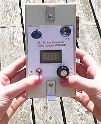 |
| Figure 22. Two-channel LED-based visible light sun photometer. |
The output voltage from the transimpedance amplifier is proportional to the amount of sunlight reaching the detector:
V = Vo(ro/r)2e-[αa + αR(p/po)]m
Solving for aerosol optical thickness (αa),
αa = [ln(Vo(ro/r)2) - ln(V) - αR(p/po)m]/m
where ln is the natural (base e) logarithm, r is the Earth-sun distance at the time of a measurement, ro is the average Earth-sun distance (1 astronomical unit), and p/po is the ratio of actual barometric pressure (station pressure) at the observing site to standard sea level barometric pressure (1013.25 mbar).
The relative air mass (m) is a measure of the path length through the atmosphere, as illustrated in Figure 23. If the sun is directly overhead, m = 1. Otherwise, m is approximately proportional to 1/sin(θ) where θ is the solar elevation angle.
 |
| Figure 23. Solar elevation angle and relative air mass. |
In the equation for aerosol optical thickness, the optical thickness due to molecular absorption (mostly ozone) is also included in "a. That is, the equation separates the total atmospheric optical thickness into two components. Molecular (Rayleigh) scattering is a quantity that depends only on barometric pressure at the observing site. The calculated Rayleigh coefficient is multipled by the ratio of the actual pressure at the observing site to sea level pressure for a standard atmosphere (1013.25 mb).
The second component of optical thickness includes molecular absorption and scattering by aerosols; this component is the purpose of the sun photometer measurement. The contributions due to ozone (and perhaps other absorbing gases under some circumstances) and aerosols can be separated after the fact, either by using climatological and latitude-dependent average ozone values, for example, or by using actual total column measurements for the time and place of the data collection. Satellite-based instruments such as the Total Ozone Mapping Spectrometer (TOMS) are sources of such data. For the GLOBE two-channel sun photometer, a typical ozone contribution to the non-Rayleigh optical thickness is about 0.01 for the green channel and 0.03 for the red channel.
The quantity Vo is the calibration constant for the instrument. It is the voltage output the instrument would produce if there were no atmosphere between the detector and the sun. Obviously, it is not practical actually to measure the voltage outside the atmosphere. However, it is possible to infer what this voltage would be. If a sun photometer views the sun through various values of relative air mass, and the total atmospheric optical thickness does not change, then the logarithm of the instrument voltage is proportional to relative air mass. By fitting a straight line through the data (a linear regression), the intersection of that line at the y-axis where m = 0 is the logarithm of the voltage the instrument would produce if there were no atmosphere. This is called a Langley plot calibration, named after Samuel P. Langley, the scientist who developed this technique in the early 20th century. (This work is described by Abbott and Fowle [1908], as part of early 20th century efforts to determine "the solar constant of radiation.")
It is not easy to do these calibrations, because it is not easy to find observing sites at which total atmospheric optical thickness remains constant for several hours, as is required to collect data over a range of relative air mass values. High elevation sites such as Mauna Loa Observatory in Hawaii are favored for such work because of the clean skies and stable meteorology at this site. Figure 24 shows a Langley plot calibration performed on a GLOBE sun photometer at MLO on June 21, 2000 [unpublished data by Brooks and Mims, 2000].
 |
| Figure 24. An example of a Langley plot sun photometer calibration. |
The logarithm of the voltage at m = 0 is 0.62238. This gives a voltage of 1.86336. The value Vo should be normalized to an average Earth-sun distance (1 AU). On June 21, the Earth-sun distance was 1.01631 AU. (Yes, it is true that Earth is farthest from the sun in the northern hemisphere summer.) The intensity of radiation from the sun, and hence the voltage, varies as the square of the Earth-sun distance, so
Vo = (1.86336)(1.01631)2 = 1.92464
That is, if the instrument were 1 AU from the sun, the voltage would be larger than it was on June 21.
Sun photometers used in the field can be calibrated by comparing their output side-by-side with a reference instrument on which a Langley plot calibration has been performed. This is called a transfer calibration. All sun photometers in use by GLOBE schools are calibrated in this way.
 |
| Figure 25. Normalized leaf transmission and LED responses for monitoring photosynthetically active radiation (from Mims, 2003). |
For an inexpensive alternative, it is possible to use the weighted sum of outputs from two LEDs -- one that responds to red light, at one end of the visible spectrum, and another that responds to blue light, at the other end. Figure 25 shows the normalized transmission of sunlight through a green poinsettia (euphorbia pulcherima) leaf, along with the response of some typical blue and red LEDs. Note that the leaf transmits green light, but absorbs a great deal of the light at red and blue wavelengths. By combining the output from blue and red LEDs, it is possible to build an instrument that agrees reasonably well with more expensive PAR sensors. Such an instrument has been described by Mims [2003]. A four-year time series of comparisons is shown in Figure 26.
 |
| Figure 26. Time series of solar noon observations of PAR at Seguin, Texas, USA, measured by a commercial sensor and by a blue-red LED pair [from Mims, 2003]. |
The water vapor instrument developed with funding from NASA's Langley Research Center is physically identical to the visible-light sun photometer shown in Figure 22 [Brooks et al., 2003]. Only the detectors are different (near-IR rather than visible). Recall that water vapor molecules absorb solar radiation at specific wavelengths. As a result, one way to determine PW is to measure the ratio of directly transmitted sunlight at two wavelengths, one inside a water vapor absorption band and one outside the band. As long as the transmission of sunlight at each of these two wavelengths is not affected differentially by some other atmospheric constituent, this ratio should be related to PW.
Figure 27 shows, first of all, the spectral variation of insolation for a standard atmosphere across the near-IR part of the solar spectrum, with the sun directly overhead. Note the water vapor absorption band centered around about 940 nm and a smaller band around 820 nm.
 |
| Figure 27. Water vapor absorption bands in
the near-IR and normalized response of two near-IR LED detectors. |
Figure 27 also shows the normalized spectral response of two possible near-IR LED detectors. In his original design for a sun photometer to measure PW, Mims [1992] suggested the use of used two IR LEDs. However, Figure 25 illustrates some of the problems arising from using detectors whose response cannot be tailored for a specific application. It would be better if the peak response of the IR1 detector were around 870 nm rather than located right over the small water vapor absorption band around 825 nm. It would be better if the peak response of the IR2 detector were centered around 940 nm rather than around 920 nm. It would be better if the response bandwidth of the IR1 detector were smaller than it is, to limit the influence of other atmospheric effects. So, for this instrument, it appears desirable to replace especially the IR2 detector with a filtered photodiode that has a peak transmission around 940 nm. The disadvantages of filters have been noted in section 2.4 but there may be no reasonable alternative to using at least one filtered photodiode in this case.
The standard way to present PW values is to convert them to the corresponding values at a relative air mass of 1. An approximate conversion when elevation angles are not too low is:
PWm=1 = PWmsin(solar elevation angle)
There are several ways to measure PW, including direct sampling from balloon-borne instruments. Reitan [1963] developed an approximate relationship between PW and dewpoint temperature:
ln(PW) = -0.981 + 0.0341Td,°F
where ln(PW) is the natural logarithm of the column water vapor in centimeters and Td,°F is the dewpoint temperature in degrees Fahrenheit. For temperature expressed in degrees Centigrade,
ln(PW) = -0 981 + 0.0341 (Td9/5 + 32) = 0.1102 + 0.0614Td
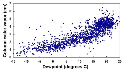 |
| Figure 28. PW calculated from dewpoint temperature, using Reitan's formula. |
Figure 29 shows how GPS-based measurements of water vapor can be used to calibrate the water vapor instrument described here.
 |
| Figure 29. Calibrating the WV instrument using GPS data. |
There are no GPS sites within a few kilometers of Philadelphia, Pennsylvania, so this is not an ideal calibration site. However, there are two sites several tens of km from Philadelphia, one to the west and one to the south. As shown by the heavy pair of lines in Figure 26, the sites give similar, but by no means identical, PW values.
As noted above, processed PW data are always given relative to the atmosphere directly over the observer (a relative air mass of 1). In order to compare these values with the ratio of two IR detectors in a sun photometer, the overhead PW values are converted to their values along the relative air mass m viewed by the sun photometer:
PW(path) = mPW(overhead)
These converted values are the light pair of lines in Figure 26. The IR detector ratios, IR2/IR1, are the lower sets of blue "x's" and "+'s" on Figure 26. With an appropriate model (roughly linear over this limited range of values), the IR2/IR1 ratios can be related directly to the PW values along the path between the observer and the sun. In Figure 26, the data are modeled against the average of the two GPS sites and the results are shown as the green "x's." If such a model can be applied over an appropriate range of PW values, then the instrument is calibrated against an independent source of PW data.
 |
| Figure 30. 2005 water vapor data from a GPS-MET site at Isabela, Puerto Rico, and Ramey School, Aguadila, Puerto Rico. |
It is not easy to measure UV radiation accurately. However, blue LEDs (which are much more recently developed devices than the widely known red, green, and amber LEDs) detect light in the near-UV, providing an opportunity for making some kinds of UV measurements with inexpensive instruments.
 |
| Figure 31. Spectral response of an unfiltered blue LED detector. |
 |
| Figure 32. UV-A detector assembly, without Teflon diffuser. |
The basic reason for developing this instrument is to support some of the data products resulting from measurements made by instruments on NASA's EOS/Aura spacecraft. These include UV radiation at Earth's surface and the total amount of ozone in the atmosphere under the spacecraft. The effects of clouds on UV radiation reaching the surface seriously impact the calculations required to develop these data products, and ongoing ground-based measurements are required in order to validate the performance of data-processing algorithms. Direct sunlight and the optical depth at UV-A wavelengths are also needed. The value of an inexpensive instrument that will meet these needs has led NASA's Goddard Space Flight Center to support development of the instrument shown here.
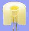
The LED detector assembly is covered with a Teflon® disk to diffuse sunlight, similar to what was used for the pyranometer. This assembly is then attached to the top of the instrument enclosure, as shown in Figure 32. The dark ring around the detector prevents light from leaking through the sides of the housing. The ring can be removed and replaced by a collimating tube with a small hole at one end (the end with the white cap in Figure 32). This tube fits snugly over the housing, giving the detector a field of view identical to the sun photometers discussed previously. Thus, a single instrument can be used to measure either full-sky or direct sun radiation. This is a useful complement to the shadowband radiometer mentioned previously, which measures full-sky and diffuse sun radiation, from which direct radiation can be calculated.
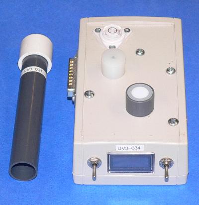 |
| Figure 32. GLOBE/GSFC UV-A radiometer and sun photometer. |
In its direct sun mode, the UV instrument can be calibrated as a sun photometer according to the discussion in a previous section dealing with aerosols. The fact that its spectral response (with the low-pass filter) is quite narrow is an advantage, because sun photometers are supposed to respond to sunlight over only a narrow spectral range. The peak response at about 372 nm is very close to the 368 nm channel on the Yankee Environmental Systems UV Shadowband Radiometer, a widely used research-quality radiometer with several channels. Thus, the instrument shown here can be calibrated, in units of W/m2, against this much more expensive instrument.
This calibration strategy assumes that the output of the LED-based UV-A instrument depends only on the intensity of the incident radiation within its spectral response, and not on detector temperature. This is an important question because of how the instrument is used. The output of all photodetectors is somewhat temperature dependent. This is not a serious problem for sun photometer measurements because measurements with a handheld instrument require only a few minutes, and it is feasible to keep the detectors at a reasonably constant temperature (around 20-25ºC) throughout the entire short procedure. On the other hand, the UV-A radiometers are typically used over much longer measurement times (~1 hour) because temporal variability of UV-A radiation due to, for example, changing cloud patterns, is of great interest for ground validation measurements that support space-based instruments. So, temperature sensitivity is a potentially serious concern.
Expensive radiometers use heaters to actively maintain the detector at a constant temperature, typically 40ºC. This is not feasible for a battery-powered handheld instrument. The UV-A radiometer described here includes a temperature sensor mounted on the top of the instrument case in a housing the same size as the detector housing, and made from the same material (nylon). (See the housing toward the rear of the instrument shown in Figure 32.) The idea is that the sensor inside this second housing will be at approximately the same temperature as the detector inside its housing. Thus, a temperature correction can be applied if necessary. Figure 33 shows voltage outputs from this radiometer. The data were collected in late morning, local time, under a partly cloudy and therefore very "noisy" sky, as indicated by the UV-A detector output in the bottom trace. (These are the weather conditions of most interest to the EOS/Aura project mentioned previously.) The upper trace is output from a temperature sensor whose output is equal to the temperature in Celsius divided by 100. On this occasion, the sensor temperature rose by about 15ºC over 20 minutes. However, there is no visible sign of a significant temperature effect on the UV-A output. (The slow rise in the UV-A output level over the entire data collection period is due to the fact that the sun is still rising in the sky.)
 |
| Figure 33. Outputs from a GLOBE UV-A radiometer. |
The measurements described above require that the position of the sun above the horizon (its elevation angle) or, equivalently, its angular position from the zenith, be accurately known. (The zenith angle equals 90º minus the elevation angle.) This is true even for full sky measurements, as their interpretation may depend on solar position.
It is possible to measure the solar elevation or zenith angle directly by, for example, measuring the length of a shadow cast on a horizontal surface by a vertical rod of known length. However, it is a better idea to calculate the position based on the time and longitude-latitude coordinates at which a measurement is taken. This reduces the work required of an observer and can be done at any time before or after a measurement. The appropriate application of astronomical equations makes this a very accurate calculation -- more accurate than can be obtained by a casual observation. The equations presented below are from a well-known book on astronomical calculations by Belgian author Jean Meeus [1991].
First, here is an algorithm that expresses calendar dates in terms of the Julian Day (JD). This provides a unique value for every day and is commonly used as the basis for astronomical calculations involving dates and times.
Given a date expressed as a month (m), day (d), and 4-digit year (y),
if m ≤ 2, subtract 1 from the year and add 12 to the month
A = <y/100>
B = 2 - A + <A/4>
JD = <365.25·(y + 4716)> + <30.6001·(m + 1)> + d + B - 1524.5
Expressions written as <...> are interpreted as "the truncated (rather than rounded) integer value of..." Thus, <8/3> = 2. Julian Days start at noon, Universal Time. Here's an example:
m = 11 d = 30 y = 2003 UT = 00:00:00 (start of calendar day)
A = <2003/100> = 20 B = 2 - 20 + 5 = -13
JD = <365.25·6719> + <30.6001·12> + 30 - 13 - 1524.5
= 2454114 + 367 + 30 - 13 - 1524.5 = 2452973.5
The day (d) can have a fractional part. If d = 30.75, the fractional part corresponds to (0.75)(24) = 18 hours, or 6 pm on November 30. The Julian day for this time is 2452973.5 + 0.75 = 2452974.25.
The next step is to calculate the position of the sun as viewed from Earth. A detailed discussion of these somewhat involved calculations is beyond the scope of this document, and can be found in Meeus [1991]. The calculations defined here imply an accuracy that may look like "overkill" for this problem. However, even simpler versions of these calculations require a computerized implementation in a program or spreadsheet. So, once the initial work of entering the equations has been done, there is no extra work associated with calculations done to this precision. Also, less precise representations of the equations can lead to cumulative errors when positions are projected far into the future (or past).
The first set of calculations gives the Earth/sun distance (R) and the longitude of the sun in ecliptic coordinates.
T = (JD-2451545.0)/36525.0
Lo = 280.46645 + 36000.76983T + 0.0003032T2
M = 357.52910 + 35999.05030T - 0.0001559T2 - 0.00000048T3
e = 0.016708617 - 0.000042037T - 0.0000001236T2
C = (1.914600 - 0.004817T - 0.000014T2)·sin(M)
+ (0.019993-0.000101T)·sin(2M) + 0.000290·sin(3M)
Ltrue = (Lo + C) mod 360
f = M + C
R=1.000001018·(1 - e2)/[1 + e·cos(f)]
These equations give angular values in degrees for Lo, M, C, Ltrue, and f. Note that trigonometric functions in computer programming languages and spreadsheet functions typically expect angles to be expressed in radians, not degrees. So, when M and f are used as arguments in a trigonometric function, they should almost certainly be converted to radians:
radians = (degrees)(π/180)
Next, calculate the mean sidereal time, the angular position (hour angle) of the point where the ecliptic plane intersects the equator.
sidereal=280.46061837 + 360.98564736629 (JD-2451545) + 0.000387933 T2
- T3/38710000
sidereal --> sidereal mod 360
Next, calculate the obliquity of the ecliptic, that is, the angle between the equatorial and the ecliptic planes.
obliquity = 23 + 26/60 + 21.448/3600 - (46.8150/3600)T - (0.00059/3600)T2 + (0.001813/3600)T3
Finally, convert the sun's position from ecliptic to Earth equatorial (longitude and latitude) coordinates.
right ascension = arctan[tan(Ltrue) cos(obliquity)]
declination=arcsin[sin(obliquity sin(Ltrue)]
hour angle=sidereal + observer longitude - right ascension
azimuth = arctan(y/x) where
y = sin(hour angle)
x = cos(hour angle) sin(observer latitude) - tan(declination) cos(observer latitude)
The warning about trigonometric functions expecting angles expressed in radians still applies. Note that the azimuth needs to be expressed as a value between 0º and 360º, or -180º and 180º. To do this, consider that the tangent of an angle is y/x. Typically, programming languages and spreadsheets include arctangent functions that require both the x and y coordinates to be specified so the function can consider the sign of each component to determine the proper quadrant for the result.
elevation (radians) = arcsin[sin(observer latitude) sin(declination) +
cos(observer latitude) cos(declination) cos(hour angle)]
zenith = 90º - elevation (degrees)
The relative air mass is defined by the solar elevation or zenith angle. It is approximately 1/sin(elevation). At an elevation angle of 90º, this expression is no longer mathematically defined. Also, as the sun gets closer to the horizon, Earth's curvature and the refraction of the atmosphere impose corrections on this simple formulation. For example, because of atmospheric refraction, the sun is still visible even when it is physically below the horizon. Here is a formulation by Young [1994], in terms of solar zenith angle (z), that does not become undefined at 90º, and that takes into account curvature and refraction:
m = [1.002432 cos(z)2 + 0.148386 cos(z) +0.0096467]/ [cos(z)2 + 0.149864 cos(z)2 + 0.0102963 cos(z)+0.000303978]
The large number of significant digits represented in the equation guarantees the "good behavior" of the function when the sun is near the horizon, but it does not imply that the calculation of m is actually this precise.
Figure 34 shows solar elevation and azimuth angle, plus relative air mass, as a function of Universal Time for a location at 75ºW longitude and 40ºN Latitude (Philadelphia, PA, USA), on 21 June, 2003, near the summer solstice. Azimuth is measured clockwise from north. In the summer, the sun at 40º north latitude rises north of due East. The sun crosses the local meridian at local solar noon (by definition) at an elevation angle of about 73.5º. In general, local solar noon is not the same as clock noon. The sun is still south of the site, because the solar declination is never more than about 23.5º north of the equator. (90º - (40º - 23.5º)) = 73.5º. Based on its definition, azimuth changes sign at noon and becomes -180º as it crosses the observer's meridian. In the evening, the sun sets north of due West. At local solar noon, the relative air mass has a minimum value of 1/sin(73.5º) = 1.043. (It never reaches a value of 1 because the sun is never directly overhead at 40ºN latitude.
 |
| Figure 34. Solar azimuth and azimuth angles, and relative air mass near Philadelphia, Pennsylvania, USA, 21 June 2003. |
The reason that local solar noon is not the same as clock noon (even at the Greenwich Meridian) is that Earth has a slightly elliptical orbit around the sun. Clock time is based on a fictitious mean sun -- a mathematical construction rather than a real object -- that "rotates" around Earth. It has the same apparent orbital period as the real sun (one year), but lags or leads the sun during the year. The so-called equation of time describes the relationship between the real and mean suns. Meeus [1994] gives this calculation for the equation of time E, in radians:
y = tan2(obliquity/2)
E = y sin(2Lo) - 2e sin(M) + 4ey sin(M) cos(2Lo) - 0.5y2 sin(4Lo) - 1.25e2 sin(2M)
It may seem strange to express "time" as an angle. However, the two are related due to the fact that Earth rotates 360º in 24 hours of mean solar time. So, 15º equals one clock hour. To express the equation of time in minutes, convert E to degrees (multiply by 180/π), divide by 15 to get the fraction of an hour, and multiply by 60. E is plotted in units of minutes in Figure 35 for 2003.
 |
| Figure 35. The equation of time for 2003. |
To find local solar noon relative to clock noon, first subtract the quantity (longitude mod 15) hours, where longitude is negative to the west. (A "mod" function returns the remainder from division. For example, (77.5 mod 15 returns 2.5) Then subtract the equation of time value E. Here's an example: When is local solar noon at 80ºW longitude on November 28, 2003?
E = 0.053785 radians = (0.053785)(180/π)(60/15) = 12.32 minutes
(-80 mod 75) = -5
local noon = 12 hours, - (-5/15)(60) - 12.32 minutes =
12 hours + (20 - 12.32) minutes = 12 hours, 7.68 minutes = 12:07:41
As shown in Figure 1, the sun behaves approximately like a blackbody -- a perfect radiator -- at a temperature of about 5800K. It is of interest to understand the source of the blackbody radiation curve shown along with the measured extraterrestrial insolation in this figure. The calculations are based on Planck's law, first published in 1901.
E = (2πhc2λ-5)/[exp(hc/λkT) 1] Δλ
where E is radiated power per unit area in the wavelength interval Δλ; λ is wavelength in meters; c is the speed of light, 2.9979 x 10⁸ m/s; h is Planck's constant, 6.6261E-34 Joule-s; k is Boltzmann's constant, 1.38065x 10⁻²³ Joule/K; T is temperature in Kelvins.
The total power radiated in the interval Δλ is 4πr2E, where the sun's radius r is about 6.96 x 10⁸ m. At the average Earth-sun radius R, the extraterrestrial radiation in the interval Δλ is E(r2/R2) W/m2, where R is about 1.5 x 10¹¹ m.
Planck derived this famous equation in an attempt to reconcile the behavior of blackbody radiation as then described by the 19th century Rayleigh-Jeans and Wien's laws. The Rayleigh-Jeans law explained blackbody radiation at long wavelengths, but not at short wavelengths. Wien's law worked for shorter wavelengths, but not for longer wavelengths. The Rayleigh-Jeans law had a firm foundation in electromagnetic theory as it was understood at the time, so its breakdown at short wavelengths (the "ultraviolet catastrophe") was profoundly disturbing to physicists.
When Planck searched for a mathematical description that would work for all wavelengths, he found that the available data on blackbody radiation could be explained by assuming that radiation is emitted only in discrete packets with an energy proportional to the inverse of wavelength: energy = hc/λ. Planck considered this assumption to be only a "fudge factor" that provided an empirical explanation of blackbody radiation. However, other physicists soon realized that this assumption must, in fact, have a physical basis that required a fundamentally new theory of electromagnetic radiation. In 1905, Einstein published a Nobel-prize-winning paper showing that the well known photoelectric effect, in which light striking certain surfaces causes a small current to flow, cannot be explained by classical theories of electromagnetic radiation, but can be explained by assuming that light energy is quantized -- transmitted only in discrete units by what are now called photons. However, the new explanation of the photoelectric effect appeared to be inconsistent with well known optical effects such as interference patterns. Such effects are completely consistent with classical theory, which attributes wavelike properties to light and other forms of electromagnetic radiation. The realization that electromagnetic radiation must have both wavelike and particle-like properties, no matter how counterintuitive such a conclusion seemed, revolutionized physics and led to the development of what is now known as quantum mechanics.
This report has provided an introduction to Earth's atmosphere, how it affects the transmission of sunlight to the surface, and how to design relatively simple instruments to measure solar radiation and, indirectly, some important atmospheric constituents. The primary target of the report is educators, including middle and secondary school students as well as college and university students. The instruments described here are, at the very least, excellent instructional tools that infuse students with a sense of how the measurement process works. Although there is a place in science education for pre-packaged, "student friendly" measurement tools and projects, students gain a sense of ownership and an entirely different perspective on science when they design and construct their own instruments. They will also gain a better appreciation of the essentially analog world of scientific measurement, a perspective that is especially important in the overwhelmingly digital environment to which students are continuously exposed.
It is important not to underestimate the difficulty of collecting reliable and accurate data in any area of science. It requires commitment, patience, and great care. In a formal educational setting, the growing need to meet very specific teaching and learning standards means that finding time for innovative hands-on, inquiry-based activities presents a serious challenge for even the best teachers.
Educational challenges aside, it is also important not to underestimate the value of data collected with the relatively inexpensive instruments described here. If they are carefully constructed, properly calibrated, and used under appropriate conditions, these instruments can produce (and have produced) scientifically useful data. Ongoing student and professional testing with these instruments show consistently good agreement with their more expensive counterparts. In particular, the performance of the visible-light sun photometers, which have been in use longer than the other instruments described here, has been confirmed through extensive comparisons with other sun photometers, such as the CIMEL sun photometers that comprise the Aerosol Robotic Network (AERONET) [Holben, et al., 1998; Brooks et al., 2003].
Because of the importance scientists attach to matters of instrument calibration and data collection, it is essential to develop partnerships with scientists who can work with both educators and students to ensure the quality of the data they collect. Beyond the data collection process, it is also important to help students understand and appreciate what they are doing. Most science educators, regardless of their teaching skills, lack research interests of their own. As a result, they are generally poorly prepared to show students how to develop their own research agendas.
It is rare to find adults, including educators, who have the basic electronic construction skills needed to build the instruments described here. Nonetheless, this is a worthwhile and empowering experience for students and educators. There are a number of books that present the basics of electronic construction. (See, for example, Mims [2003].) With adequate supervision, this kind of work is certainly appropriate for secondary and some middle school students.
It is usually inefficient and relatively expensive to purchase parts for making just one or two instruments because electronics suppliers invariably favor purchases in quantity. In any event, it is a better idea to get enough parts for several instruments, especially in situations where inexperience will invariably lead to mistakes. In some cases, detailed instructions and/or complete kits of parts are available for building the instruments described here. Contact the author at the e-mail address given on the title page of this document.
This paper is based on work made possible by grants and other support from the GLOBE Program (through the National Science Foundation), NASA Goddard Space Flight Center, and NASA Langley Research Center.
Anyone who is interested in these kinds of measurements and instruments is deeply indebted to the groundbreaking and continuing work by Forrest M. Mims III, the inventor of LED-based instruments for atmospheric measurements, and Co-Principal Investigator for the GLOBE Program's Aerosols, Water Vapor, and UV-A Monitoring Projects. Forrest has been a professional inspiration, a valued colleague, and a personal friend since beginning our work together with the GLOBE Program in 1998.
Some of the figures in this document were originally prepared by Schafer-LaCasse Design for the GLOBE Program.
Abbott, C. G., and F. E. Fowle, Jr., Annals of the Astrophysical Observatory of the Smithsonian Institution, Vol. II, Part 1, 11-124. US GPO, Washington, DC, 1908.
American Chemical Society, Chemistry in Context: Applying Chemistry to Society. 2000.
Bird, R., and C. Riordan, Simple Solar Spectral Model for Direct and Diffuse Irradiance on Horizontal and Tilted Planes at the Earths Surface for Cloudless Atmosphere. Solar Energy Research Institute SERI/TR-215-2436, 1984. (online at rredc.nrel.gov/solar/pubs/spectral/model.)
Brooks, D. R., and F. M. Mims. III, Development of an inexpensive handheld LED-based Sun photometer for the GLOBE program. J. Geophys. Res. 106(D5), 4733-4740, 2001.
Brooks, David R., F. Niepold, G. DEmilio, J. Glist, G. Hatterscheid, S. Martin, K. Dede, I. Neumann, Scientist-Teacher-Student Partnerships for Aerosol Optical Thickness Measurements in Support of Ground Validation Programs for Remote Sensing Spacecraft. 54th International Astronautical Congress, Bremen, Germany, Sept. 28 - Oct. 3, 2003.
Brooks, David R., Forrest M. Mims III, Arlene S. Levine, Dwayne Hinton, The GLOBE/GIFTS Water Vapor Monitoring Project:An Educator's Guide with Activities in Earth Sciences. NASA Publication EG-2003-12-06-LARC, 2003.
Bucholtz, Anthony, Rayleigh-scattering calculations for the terrestrial atmosphere. Applied Optics, 34, 15, 2765-2773, 1995.
Diak, G. R., W. L. Bland, and J. R. Mecikalski, et al., A note on first estimates of surface insolation from GOES-8 visible satellite data. Agricultural and Forest Meteor. 82, 219-226, 1996. (See http://homer.ssec.wisc.edu/~insol/.)
Holben, B. N., et al., AERONET -- A federated instrument network and data archive for aerosol characterization, Remote Sensing of the Environment, 66, 1-16, 1998.
J.D. King, J. D., and D.R. Myers, Silicon-Photodiode Pyranometers: Operational Characteristics, Historical Experiences, and New Calibration Procedures, 26th IEEE PV Specialist Conference, 1997, pp. 1285-1288.
Mims, Forrest M., III, Sun photometer with light-emitting diodes as spectrally selective detectors. Applied Optics, 31, 33, 6965-6967, 1992.
Mims, Forrest M. III, An inexpensive and stable LED Sun photometer for measuring the water vapor column over South Texas from 1990 to 2001, Geophys. Res. Lett., 29, 13, pp 20-1 -- 20-4, 2002.
Mims, Forrest M. III, Getting Started in Electronics, Master Publishing, Lincolnwood, IL, 2003.
Mims, Forrest M. III, A 5-Year Study of a New Kind of Photosynthetically Active Radiation Sensor. Photochemistry and Photobiology, 77, 1, 30-33, 2003.
Meeus, Jean, Astronomical Algorithms. Willmann-Bell, Richmond, Virginia, 1991.
Reitan, C. H., Surface Dew Point and Water Vapor Aloft, J. Applied Meteorology, 2, 776-779, 1963.
Voltz, Frederick E., Economical Multispectral Sun Photometer for Measurements of Aerosol Extinction from 0.44 μm to 1.6 μm and Precipitable Water. Applied Optics, 13, 1732-1733, 1974.
Young, Andrew T., Air mass and refraction. Applied Optics, 33, 6, 1108-1110, 1994.